
A go/no-go decision dressed as a configuration switch
Switching from FP16 to FP8 reduces three resource categories at once: less VRAM per parameter, narrower data paths, and higher operations per joule. The configuration change is small. The decision to make the change feels small. The decision is not small. Precision reduction is an economic lever that lowers cost on three axes simultaneously and risks introducing a silent quality regression on a fourth, and the right framing is a deliberate go/no-go decision against measured evidence, not a default-on configuration toggle.
The structure of when precision reduction is worth its risk — and what the measurement contract looks like that makes the decision honestly — is the operational content of treating precision as an economic decision rather than a flag.
Which three cost axes does precision reduction lower simultaneously?
Reducing precision from a higher-bit format to a lower-bit format produces compounding cost reduction across three independent axes:
Memory footprint. Smaller per-value representations mean the model occupies less memory. A model that fits in less memory either fits on smaller (cheaper) accelerators or leaves more memory available for KV-cache, batching headroom, or co-tenant workloads. The cost effect is direct: a deployment that needs N GB of accelerator memory at FP16 needs roughly N/2 GB at FP8.
Memory bandwidth. For inference workloads that are memory-bandwidth-bound — which describes most autoregressive LLM inference under cuDNN/FlashAttention kernels, and many vision deployments running through TensorRT — the time to read weights and activations dominates the time to compute on them. Halving the per-value size halves the bandwidth requirement, which can directly translate into roughly proportional throughput improvement on bandwidth-bound workloads (observed across TechnoLynx inference-optimization engagements; not a benchmarked rate that holds universally).
Compute throughput. Modern accelerator matrix engines deliver more operations per second at lower precision when the precision is natively accelerated. Per NVIDIA’s published specifications, the peak throughput at FP8 on a Hopper-class GPU is materially higher than at FP16 on the same device.
These axes compound rather than add. A workload that benefits from all three simultaneously sees a cost-per-token reduction larger than any single axis would suggest. The economic appeal is real. The dependency structure that makes it real also creates the risk profile.
There is a flip side worth stating plainly: above the precision a given workload actually needs, extra bits buy nothing. If the lower-precision configuration meets the quality bar on the production input distribution, the higher-precision run is paying for memory, bandwidth, and compute the workload never converts into better output. In that regime higher precision is economically wasteful — not wrong, just over-provisioned — and the cost it carries is the gap between the format you are running and the lowest format that still clears your accuracy contract. Which format that is depends entirely on the workload and the SLA around it; the same model that tolerates FP8 on a noise-absorbing re-ranker may need FP16 behind a tight latency-and-quality SLO.
The fourth axis: accuracy that may degrade silently
Quality regressions introduced by lower bit-widths rarely announce themselves at deployment time; they surface only under production traffic patterns. The degradation surfaces in production, on production inputs, sometimes weeks later. Three patterns recur in the deployments we audit.
Tail-input degradation. The quantized model performs as expected on inputs similar to the calibration set and degrades on inputs outside it. A model calibrated on benchmark prompts can degrade on long-context inputs, on code, on non-English text, or on any other regime the calibration didn’t cover. The aggregate accuracy on a clean test set may look fine; the production accuracy on the actual input distribution may not.
Reasoning collapse. Models that perform multi-step reasoning can be more sensitive to quantization than single-step models because errors compound across reasoning steps. A model that quantizes cleanly on classification can fail on chain-of-thought tasks where the same numerical perturbation, propagated through reasoning, produces output divergence. This is an observed pattern across our LLM deployments, particularly with code-generation and multi-hop QA workloads.
Distribution-shift sensitivity. The quantized model’s behavior under distribution shift can differ from the full-precision model’s. A model that handles a 10% out-of-distribution shift gracefully at FP16 can degrade more sharply at FP8, because the quantization scheme was calibrated against an in-distribution sample and the out-of-distribution behavior was not characterized.
These patterns are silent in the sense that they don’t trigger errors or alerts — they produce wrong outputs that look like normal outputs. A buyer who deploys quantization without measurement against the production input distribution is exposed to this class of regression, and the cost-saving math does not include the cost of the regression.
The break-even framing
Frame the tradeoff as equilibrium: at what accuracy penalty does the infrastructure discount become uneconomical? That calculation defines the decision boundary.
The cost saving is measurable. The accuracy loss has to be measured to be known. Without the second measurement, the break-even cannot be calculated, and the decision is being made by assuming the accuracy loss is zero (or small, or acceptable) on no evidence.
The framing requires:
- Cost saving quantified for the specific deployment: memory, bandwidth, throughput, energy, accelerator-instance count.
- Accuracy loss quantified for the specific (model, task, quantization scheme) on the buyer’s workload, evaluated on a representative input distribution including likely edge cases.
- Cost of accuracy loss quantified in terms the business can compare to the cost saving — user-facing quality impact, error rate against SLO, downstream impact on dependent systems.
When all three are quantified, the break-even is computable. When the accuracy loss or its business cost is unmeasured, the decision is being made on partial evidence and the result depends on whether the unmeasured part happens to favor the choice or not. This is where the broader argument for precision as an economic lever in inference systems becomes operational rather than abstract.
Where the throughput half of the trade comes from
Cloud providers now expose per-request cost metrics through standard APIs, eliminating the need for specialized profiling hardware. A 26Q3 LynxBenchAI run reports per-precision behaviour across the catalogue and weights throughput by the memory a run actually moves, so a cheap-looking low-precision result has to earn its speed-up rather than be credited for being cheap. The run discards a warm-up phase and counts completed iterations inside a continuous timed window, at a workload already scaled until throughput stops improving — which is what makes the number a sustained figure rather than a burst reading. Results arrive as Training, Inference, and Compute plus GT, an ordinal aggregate over the three category scores, so a precision decision stays attached to the class of work being paid for rather than to an undifferentiated rating. Installation is pip install lynxbench-ai, roughly 15–30 minutes to a result, Personal Edition free for non-commercial use.
What the run does not give you matters just as much before the number enters a spreadsheet. It covers a fixed catalogue under one named release; it is not a price, not a cost-per-request figure, and not a stand-in for your bill. It does not record conditions it never measured — thermal state among them. And 26Q3 figures are not comparable against another release name: 26Q3 is current, 27Q1 is next, and that is a naming scheme rather than a schedule. Converting a throughput figure into currency is the reader’s step, taken with those bounds stated rather than assumed.
When precision reduction is a clear win
Some deployment contexts make precision reduction a near-default choice with low risk:
- Workloads where the accuracy delta is reliably small. Specific (model, task) combinations are well-characterized as quantization-tolerant — many vision classification models running through TensorRT, well-conditioned LLMs on standard tasks, embedding models with margin to spare. Measurement still required, but the prior is favorable.
- Cost-dominated economics. Deployments where the cost saving is large enough that even a modest accuracy degradation is worthwhile. High-volume inference at marginal cost is the typical case.
- Tolerant downstream systems. When the inference output feeds a downstream system that itself absorbs noise (a re-ranker, a downstream classifier with high precision/recall margin, a human-review step), small accuracy degradations may not propagate to user-facing quality.
- Recoverable-error contexts. Tasks where errors are easily detected and corrected — for instance, a fallback to a higher-precision PyTorch model invoked when a confidence threshold is breached — tolerate aggressive quantization with controllable risk.
When precision reduction is a no-go
And some deployment contexts argue for caution:
- High-stakes outputs. Medical, legal, financial, or safety-critical contexts where output errors carry asymmetric costs. The expected-value math includes a long-tail downside that may exceed any plausible cost saving.
- Reasoning-heavy workloads. Chain-of-thought, multi-step arithmetic, code generation. Compounding errors make even small per-step accuracy losses produce large output divergence.
- Distribution-shift-sensitive deployments. When the production input distribution differs from the calibration distribution in unpredictable ways, the post-quantization behavior under shift is hard to bound.
- Long-context, rare-class, or otherwise sparse-evaluation regimes. Aggregate test-set accuracy systematically misses degradation concentrated in specific input subsets, and these contexts are exactly where degradation tends to be largest.
The framing in both cases is the same: the buyer has to measure the accuracy on the actual workload before committing, and the measurement has to include the regimes the deployment will encounter, not only the regimes the off-the-shelf benchmarks happen to cover.
Precision-reduction break-even checklist
A precision-reduction proposal is decision-grade only when each of the following is documented:
- Cost saving quantified. Per-token energy, per-request latency, and accelerator-hour reduction are estimated against the current FP32/FP16 baseline on the team’s workload, not against a vendor headline.
- Accuracy delta measured on the production workload. The lower-precision configuration’s output quality is evaluated against the team’s evaluation rubric, not the calibration set.
- Per-stratum accuracy reported. Aggregate accuracy is decomposed by rare classes, edge inputs, or other strata where degradation tends to concentrate.
- Throughput figure carries its exclusions. The per-precision number names its release, its catalogue, and what it does not record.
- Business cost of accuracy regression named. Downstream cost (refunds, escalations, safety review, reputational risk) is converted into a value the cost saving must clear.
- Reversal plan documented. A path back to the higher-precision regime exists if monitoring detects a regression in production.
A proposal missing any item is a configuration toggle dressed as a decision, not a break-even case.
The framing that helps
Numerical precision trades off against three cost vectors—storage, transfer, and compute—while exposing model outputs to a creeping quality tax. The right framing is a break-even decision against measured evidence — cost saving quantified, accuracy loss quantified on the actual workload, business cost of accuracy loss quantified — not a default-on configuration toggle. Some contexts make the decision a clear win; others argue for caution; in both cases, the measurement is the contract that lets the decision be made honestly.
LynxBenchAI treats cost-relevant metrics and accuracy at each precision regime as an inseparable pair of required disclosures, because a go/no-go on precision reduction needs both halves measured against the production workload. The question worth asking of any precision-reduction proposal is whether both halves of the trade are on the table under a stated measurement contract, or only the cost-saving half?
Frequently Asked Questions
How do I decide between FP16, FP8, and INT8 for a specific deployment?
Treat it as a break-even decision, not a default. Quantify the cost saving for your deployment (memory, bandwidth, throughput, energy, accelerator-instance count) and measure the accuracy delta of each candidate format on your actual production input distribution, including edge cases. The lowest format that still clears your accuracy contract is the cost-optimal choice for that workload and SLA.
How can quantization degrade accuracy without raising any alerts?
Quantization regressions are silent because they produce wrong outputs that look like normal outputs rather than triggering errors. The common patterns are tail-input degradation outside the calibration set, reasoning collapse where per-step errors compound, and sharper degradation under distribution shift. Aggregate test-set accuracy routinely hides these because the damage concentrates in specific input strata.
When is lowering precision a clear no-go?
Hold the line on high-stakes outputs (medical, legal, financial, safety-critical) where errors carry asymmetric cost, on reasoning-heavy workloads where errors compound, on distribution-shift-sensitive deployments, and on long-context or rare-class regimes where aggregate accuracy hides concentrated degradation. In each case the long-tail downside can exceed any plausible cost saving.
What does a released 26Q3 per-precision result explicitly exclude before it can support a cost argument?
It covers a fixed catalogue under one named release and reports throughput weighted by the memory a run actually moves — it is not a price, not a cost-per-request figure, and not a substitute for your own bill. It also does not record conditions it never measured, thermal state among them, and its figures are not comparable across release names. Those exclusions have to travel with the number when it enters a break-even case.
When cutting bits cuts corners
Models compressed from FP32 to INT8 can achieve throughput multipliers of 4× and infrastructure cost cuts approaching 50%, but outlier inputs may trigger silent failure modes that evade benchmark detection. So the question to carry forward is this: do you know the executor, the rules, and the release behind the number in front of you — and if not, what would it take to find out?