When the AMD vs NVIDIA inference calculus shifts
ROCm maturity determines whether AMD undercuts NVIDIA on cost per inference; TensorRT support tilts the calculus back toward NVIDIA for compatible architectures. The vendor choice is not a static preference; it is a function of which model class, which memory footprint, and which software stack the team is willing to maintain.
That condition — “models that TensorRT supports” — covers the majority of production inference workloads we see in practice: transformer-based LLMs, ResNet-family vision models, BERT-style encoder architectures. For these model classes, TensorRT’s operator fusion, precision selection, and hardware-specific tuning typically delivers an observed range of 2–4× throughput improvement over a baseline PyTorch runtime (observed pattern across our deployment work, not a benchmarked rate). On NVIDIA hardware, that effective throughput shifts the cost-per-inference comparison further in NVIDIA’s favour than raw hardware pricing alone suggests.
Where AMD’s cost case is strongest
Single MI300X cards ship with 192 GB HBM—more than double the 80 GB in an H100 SXM and nearly twice the 94 GB in an H100 NVL. For inference workloads where the primary bottleneck is fitting the model in memory — large LLMs serving multiple concurrent sessions with long context windows — the memory capacity advantage can shift the cost calculus decisively.
A 70B parameter model at FP16 requires roughly 140 GB of GPU memory for weights alone, before activations and KV-cache. An MI300X serves that footprint in a single card. An H100 requires two cards plus NVLink, which changes both the bill of materials and the inter-GPU communication pattern. The hardware cost comparison at that model size looks different from comparisons drawn at 7B or 13B scale.
Where each platform wins on cost-per-inference
| Factor | NVIDIA advantage | AMD advantage |
|---|---|---|
| TensorRT-supported models | 2–4× throughput uplift → lower cost-per-inference (observed-pattern) | — |
| Models > 80 GB VRAM (single card) | Requires multi-GPU + NVLink | Single MI300X with 192 GB may suffice |
| ROCm-mature model architectures | — | Competitive cost-per-inference where ROCm kernels are deep |
| Software optimisation effort | Lower — larger ecosystem, more tooling | Higher — narrower ecosystem, more manual tuning |
| Team familiarity (CUDA-experienced) | Productive immediately | Switching cost in tooling and kernels |
The table is the decision surface. None of the rows are universally decisive — each one depends on the workload in front of you.
The inference question that matters
Treating AMD versus NVIDIA as a one-time platform decision ignores how quickly software support and pricing shift. The correct question is narrower: for the specific model you are serving, at the batch sizes you operate, with the software stack you are deploying, what is the cost-per-inference on each platform?
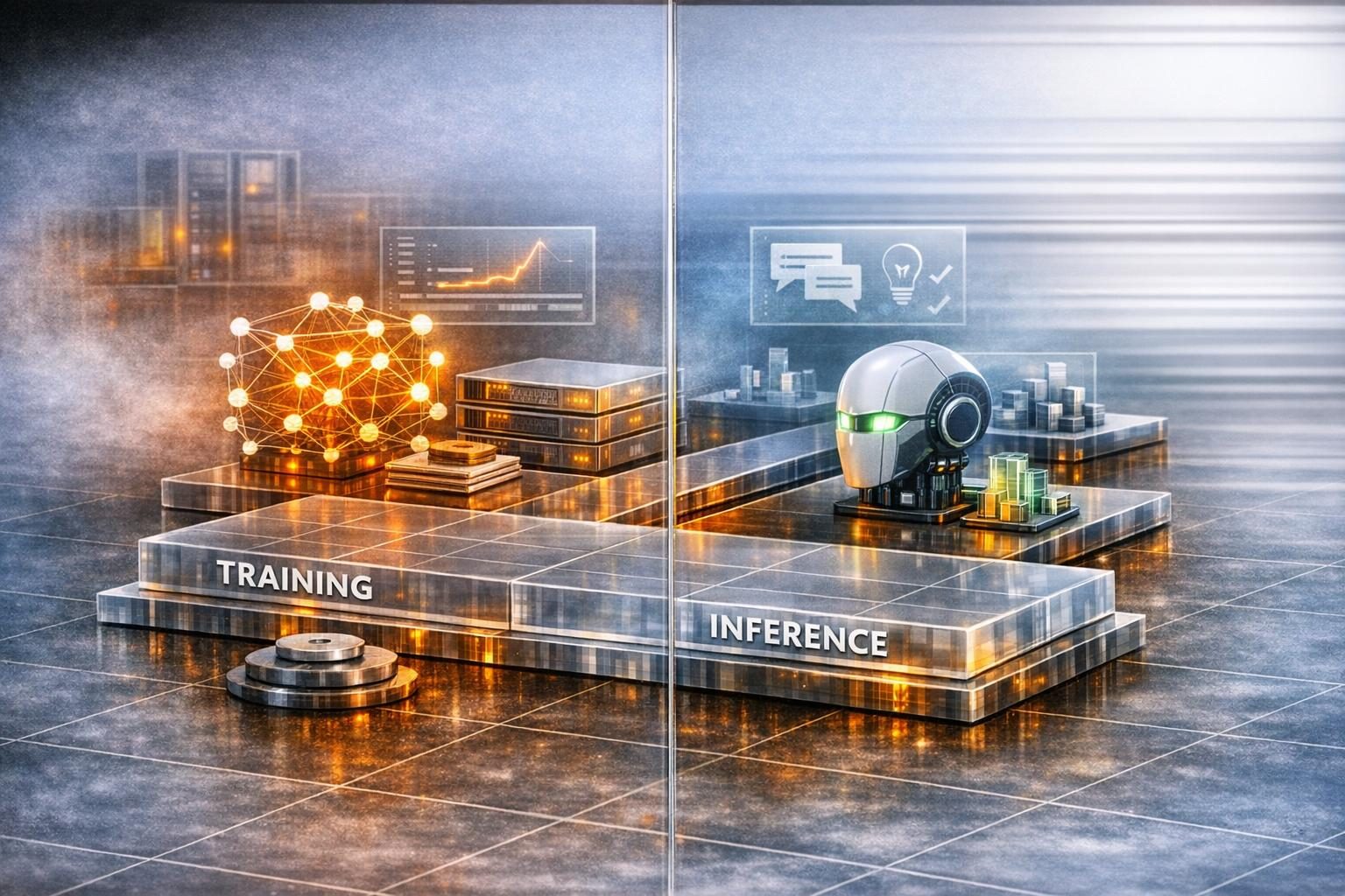
That question requires measurement. Neither vendor’s published specifications nor benchmark results from someone else’s workload will resolve it for your deployment. The two platforms handle different model sizes and architectures differently enough that no general answer carries across contexts. Understanding why training and inference create different hardware requirements — and why the comparison changes by workload type — is the deeper argument in Training and Inference Are Fundamentally Different Workloads.
How do you evaluate the true cost of switching to AMD?
List prices place MI300X roughly 20–30% cheaper than H100 at equivalent memory capacity, though procurement terms vary widely. The total cost comparison is more nuanced because software stack maturity differs significantly.
NVIDIA’s software ecosystem — CUDA, cuDNN, TensorRT, Triton Inference Server, NCCL — has had more than fifteen years of optimisation. AMD’s ROCm ecosystem is functional but less mature: fewer optimised kernels, less framework integration testing, a smaller community producing solutions to operational issues. The engineering time required to reach equivalent performance on AMD varies by workload class. For standard PyTorch training on common architectures (transformers, CNNs), ROCm delivers roughly 85–95% of CUDA’s optimised performance with minimal additional effort. For custom CUDA kernels, serving frameworks built on TensorRT plugins, or multi-GPU communication-heavy workloads using NCCL collectives, the gap widens and the engineering effort to close it grows substantial.
Our recommendation, when teams ask us to scope this: evaluate AMD hardware for workloads where the software stack is mature (standard training, large-batch inference on supported architectures), and NVIDIA for workloads requiring cutting-edge software features (FlashAttention variants, custom CUDA kernels, multi-node training with NCCL). The cost savings from AMD hardware are real, but they must be weighed against the engineering investment required to reach equivalent production performance.
Team expertise is the often-overlooked variable. A team with deep CUDA experience will be more productive on NVIDIA hardware on day one. A team starting from scratch carries less switching cost and may benefit from AMD’s lower hardware pricing. We help clients evaluate this tradeoff through a structured short-pilot pattern: deploy the target workload on both platforms, measure throughput and latency under realistic load, and calculate cost-per-inference including both hardware amortisation and engineering setup time.
Monitoring AMD GPU deployments
Observability stacks built for NVIDIA tooling do not translate directly to AMD environments. rocm-smi replaces nvidia-smi for GPU status. rocprofiler and the ROCm tracing tools replace Nsight Systems (nsys) for kernel profiling. The metrics are comparable, but the tool interfaces differ enough to require team training when transitioning from an NVIDIA environment.
We maintain parallel monitoring dashboards for NVIDIA and AMD deployments, normalised to common metrics — sustained throughput, p99 latency, power consumption, package temperature. That normalised view enables direct cost-efficiency comparison between the two platforms using production data rather than benchmark projections. Over six-month operating windows, production cost-efficiency data is consistently more informative than any pre-deployment benchmark for the next round of procurement.
FAQ
Which workload patterns favour cloud GPU rental versus owning hardware?
Bursty workloads — periodic batch jobs, training experiments, traffic with sharp diurnal peaks — favour cloud because the idle hours are not billed. Sustained workloads — always-on inference services, long-running training runs, steady-throughput pipelines — favour on-premise because the duty cycle stays high enough to amortise the hardware.
How do I model GPU total cost of ownership without guessing at utilisation?
Profile the actual workload first. Capture utilisation distributions over a representative window, not averages. Model both platforms against the observed distribution, include engineering setup time and switching cost, and let the comparison run over a 24–36 month horizon. Guesses about utilisation are the largest source of error in these models.
Three Variables That Override Brand Loyalty
Run inference benchmarks across your actual workload mix, divide total cost by delivered inferences, and let the spreadsheet settle the vendor question. For the deeper structure of that decision — utilisation patterns, amortisation windows, residency constraints — see our cloud GPU vs on-premise AI accelerators total cost analysis. The vendor question is downstream of the workload question, and the workload question is answered with profiling, not with positioning. We run that profiling pass as part of a GPU Performance Audit whenever a client is choosing between AMD and NVIDIA on a specific workload.